The Analytical Path to the Riemann Hypothesis: A Guided Expedition

Embarking on the journey to understand the Riemann Hypothesis is like climbing a mountain with several base camps. Each “base camp” represents a major area of mathematics, and along the way lie crucial “stepping stones” – intuitive concepts, theorems, and analogies – that bridge one level to the next. In this guided expedition, we will start from the very foundations (calculus and linear algebra) and ascend step by step through vector calculus, real analysis, complex analysis, the Riemann zeta function, and finally arrive at the summit: the Riemann Hypothesis itself and current efforts to prove it. At each stage, we’ll focus on intuitive, non-rigorous explanations – the kind you might find in friendly Q&A forums or vivid educational metaphors – to illuminate the key ideas without heavy formalism. Think of it as following a trail of insight, where each marker is self-contained and easy to grasp for a lay explorer. Let’s begin our ascent.

Base Camp 1: Calculus and Linear Algebra – Building the Foundation

Before tackling the heights of advanced analysis, we establish a solid base with basic calculus and linear algebra. These fields are the “oxygen and supplies” for our trek – essential tools that will support all higher reasoning.

Stepping Stone – Calculus: Understanding Change and Infinity

Calculus is the mathematics of continuous change. In calculus, we learn how to describe how quickly things change (with derivatives) and how to accumulate quantities (with integrals). For example, if distance changes over time, calculus gives us velocity and acceleration – rates of change that are intuitive in everyday life. Just as importantly, calculus introduces the concept of the limit, which lets us talk about what happens as we “zoom in” on a point or as some quantity grows without bound. This idea of tending toward a value is critical for making sense of infinite processes.

One of the most eye-opening lessons in basic calculus is dealing with infinite series – summing infinitely many terms. At first, it sounds impossible to add up infinitely many numbers and get a finite answer, but calculus (and its rigorous cousin, analysis) provides the tools to determine whether such a sum converges to a limit or diverges (grows without bound). For example, the series $1 + \tfrac{1}{2} + \tfrac{1}{3} + \tfrac{1}{4} + \cdots$, known as the harmonic series, diverges – it keeps growing slowly but inexorably to infinity[1]. This fact is surprising because the terms $\tfrac{1}{n}$ get very small, yet not small enough to prevent the infinite sum from blowing up. Such insights teach us caution and precision when handling infinity. (We’ll later see that this divergent harmonic series is intimately related to the Riemann zeta function at $s=1$ – a preview of things to come.)

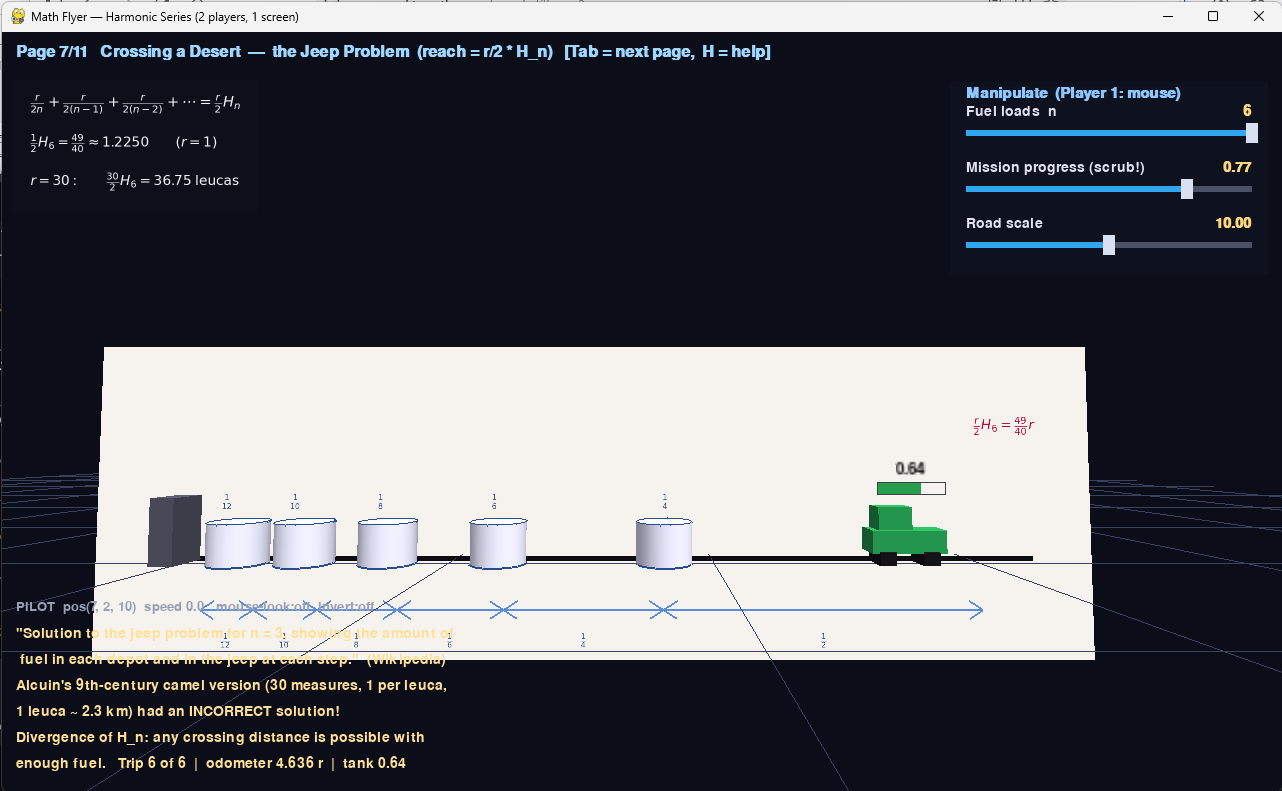
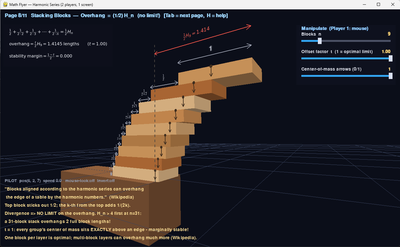
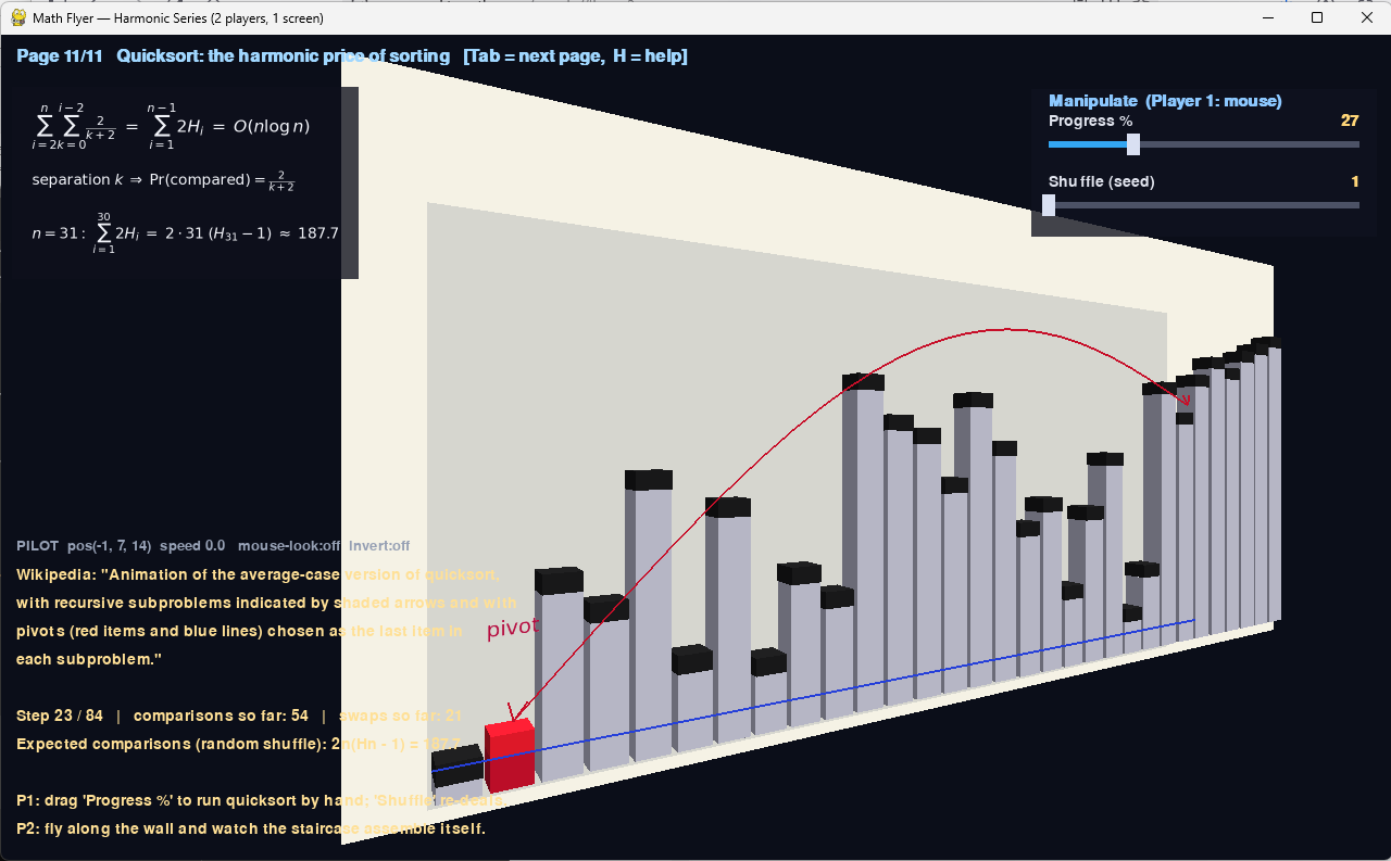
♾️ Play the Interactive 3D Demo — Two players, one screen

We built a 3D "math flyer" that turns the harmonic series into a world you can fly through together. One player pilots the camera Descent-style; the other drags Manipulate-style sliders to bend the world in real time. Tab cycles through eleven faithfully-rendered scenes — from the famous Oresme comparison test to the Quicksort sorting algorithm — each a consequence of one stubborn, divergent series.

♾️ Enter the Harmonic Series Demo →

Free & open-source — two players, one keyboard + one mouse. No signup, no payment, ever.

Another fundamental result learned early on is that some infinite series do converge to beautiful values. A famous example is the Basel Problem: the sum of the reciprocals of the squares of all positive integers, $1 + \tfrac{1}{2^2} + \tfrac{1}{3^2} + \tfrac{1}{4^2} + \cdots$, actually converges to a precise number. In 1734, the young Leonhard Euler stunned the mathematical world by finding its sum: $1 + \frac{1}{4} + \frac{1}{9} + \cdots = \frac{\pi^2}{6} \approx 1.644934$[1]. This was one of the early glimpses of the mysterious constant $\pi$ showing up in an infinite sum of rational terms – an indication that deep connections underlie even simple-looking series. This particular series is now recognized as $\zeta(2)$, the Riemann zeta function evaluated at $2$, although Euler solved it long before Riemann generalized the zeta function. The Basel Problem taught mathematicians that infinite processes, handled with care, can yield exact results and that new mathematical ideas (like the zeta function) might be lurking in familiar territory.

In short, calculus gives us the mindset and techniques to handle continuous change and infinite processes. We gain intuition for how something can approach a value ever more closely (but perhaps never exactly reach it) and how an infinite summation can sometimes make sense and equal a finite number. These concepts of convergence, divergence, and limit processes form the bedrock for later understanding the convergence of the Riemann zeta series and the idea of extending functions beyond their naively defined domain. We’ll carry these fundamental tools as we climb.

Stepping Stone – Linear Algebra: The Language of Mathematical Structures

If calculus is about change, linear algebra is about structure. Linear algebra teaches us how to work with vectors (quantities with multiple components) and matrices (arrays of numbers that linearly transform vectors). At its heart, linear algebra is the study of linear relationships – the simple, straight-line relationships that form the first-order approximation to anything. Why is this important for the Riemann Hypothesis journey? Because higher mathematics often breaks complicated problems into simpler linear pieces.

In linear algebra we learn that any linear transformation (like rotating or stretching the plane) can be understood by looking at special vectors called eigenvectors, which are vectors that a transformation merely stretches or squishes (by their eigenvalue) without changing direction. This idea of finding nice “basis” vectors that simplify a problem is everywhere in advanced math. For example, when studying vibrations or frequencies (like musical notes), linear algebra tells us that there is a basis of pure tones (sine waves) – these are eigenfunctions of the differentiation operator. This is essentially the idea behind Fourier analysis, where we decompose a complicated signal into pure frequencies. Why mention this here? Because down the road, the distribution of prime numbers will be connected to vibrations and frequencies as well – the so-called “music of the primes.” Linear algebra’s mindset of breaking things into eigen-components foreshadows the way we’ll break down the prime counting function into contributions from each zero of the zeta function (each zero acting a bit like a “note” in an orchestra, as we’ll see later[2]).

Even though linear algebra deals with finite-dimensional vectors and matrices, it lays the conceptual groundwork for thinking about spaces of functions and transformations on them (what eventually becomes functional analysis). It also introduces us to thinking in terms of multiple dimensions easily. For instance, solving a system of equations is made intuitive by thinking of each equation as a plane and a solution as their intersection. That geometric intuition in multi-dimensions will help when we move to complex numbers (which can be thought of as 2-dimensional vectors) and beyond.

To summarize, linear algebra contributes the structural and algebraic intuition: we become comfortable with abstracting problems into vectors and transformations, and finding convenient coordinate systems (bases) to simplify them. As we proceed upward, this perspective will be valuable when grappling with complex functions and their symmetries. It’s like having a good sense of direction and coordinate maps during our climb – it helps orient us in the more rarefied air of advanced topics.

Up next: Armed with the basic understanding of continuous change (calculus) and structural reasoning (linear algebra), we move to multivariable calculus and vector calculus, where we extend these ideas to higher dimensions and learn a crucial fact: sometimes, integrating around a boundary tells us what’s happening inside. This principle will echo later in the powerful methods of complex analysis.

Base Camp 2: Vector Calculus – Extending to Higher Dimensions

Having solid footing in basic calculus, we now venture into multiple dimensions. Vector calculus (or multivariable calculus) is like climbing from foothills to rolling hills – the terrain becomes multi-dimensional, and we need to keep track of directions and flows. In this camp, we learn how calculus generalizes when you have functions of several variables or curves and surfaces in space.

Stepping Stone – Multivariable Thinking: From Slopes to Flows

In single-variable calculus we had derivatives (slopes of curves) and integrals (areas under curves). Vector calculus introduces partial derivatives, which measure how a function changes as we vary one of many input variables while keeping the others fixed. For instance, if temperature $T(x,y,z)$ varies in space, the partial derivative $\partial T/\partial x$ tells us how quickly temperature changes as we move in the $x$-direction (east-west, say) while staying at the same $y$ and $z$. This concept generalizes slope to surfaces and higher-dimensional surfaces.

More dramatically, we get the notion of gradient, which is like a vector pointing in the direction of steepest ascent on a hill, with length indicating how steep the climb is. If you imagine a topographic map of a mountain, the gradient at a point would be an arrow on the map showing which way is “uphill” and how steep. This intuition helps when we later consider complex functions: surprisingly, complex differentiable functions behave as if they have no change in one specific rotated direction, thanks to the Cauchy-Riemann equations. But we’re getting ahead of ourselves – the key is that multivariable calculus trains us to think of functions as surfaces and to visualize rates of change in every direction.

Stepping Stone – Field Interpretation: Divergence, Curl, and Green’s Theorem

One of the gems of vector calculus is the way it relates integrals on the boundary of a region to integrals over the region itself. You learn about vector fields – imagine assigning a vector to every point in space, like a wind map giving velocity at each point. Two important operations on these fields are divergence (how much something spreads out from a point) and curl (how much something swirls around a point). These might sound technical, but here’s an intuitive picture: if you have a closed curve (like a loop) and you integrate a field along that loop (imagine walking along a closed path and adding up some component of a field), Green’s Theorem tells you this loop integral can be related to the divergence or curl of the field inside the loop.

For example, suppose water flows on a flat surface and you want to know how much rotates inside a loop – you could integrate the “circulation” around the loop or look at the curl inside. Green’s Theorem says these are two sides of the same coin. In formula form, $\oint_{\text{loop}} (P\,dx + Q\,dy) = \iint_{\text{inside}} \left(\frac{\partial Q}{\partial x} - \frac{\partial P}{\partial y}\right) dx\,dy$. The details aren’t important for us beyond recognizing a powerful principle: the behavior of a function (or field) inside a region can be deduced by integrating around the boundary. This is profound – it’s like saying you can detect what’s inside a black box by feeling around its surface.

This principle foreshadows one of the greatest tools we’ll use later in complex analysis: Cauchy’s Integral Theorem, which in spirit says that for certain nice fields (specifically, gradients of harmonic functions or fields with zero curl), the integral around a closed loop is zero. If not zero, something inside (like a singularity or source) is causing it – and Cauchy’s Integral Formula and the Residue Theorem make this precise for complex functions. In other words, vector calculus is training us to think about contour integrals and relate them to what’s inside the contour. We will soon apply this thinking to the complex plane, where it becomes an incredibly elegant way to compute difficult integrals or sums by “counting” what poles (singular points) lie inside the contour.

To put it simply, in vector calculus we learn that certain integrals are path-independent (the integral from A to B is the same along any route if there’s no “vortex” inside), and closed-loop integrals can reveal if singularities or sources are present. This idea will be instrumental when we encounter integrals of the Riemann zeta function in the complex plane – we’ll encircle regions and deduce information about zeros inside.

Next step: We’ve acclimatized to thinking in multiple dimensions and using integrals to glean interior information. Now it’s time to rigorously justify these intuitive concepts – we ascend to real analysis, where the notion of limit, convergence, and continuity are given a rock-solid foundation. Real analysis will also introduce us to deeper properties of series and functions that are crucial for defining the zeta function properly outside its initial domain.

Base Camp 3: Real Analysis – Rigorous Foundations of Calculus

Real analysis is often compared to “boot camp” in a climber’s training. It’s where we strip away any remaining hand-wavy understanding and replace it with precise definitions and proofs. In our journey, real analysis ensures that when we talk about infinite sums, limits, and continuous functions, we have unambiguous meaning. This will be crucial when extending the definition of the Riemann zeta function beyond simple cases.

Stepping Stone – Rigor and Proof: $\epsilon$-$\delta$ and Convergence

The first stepping stone in real analysis is understanding the formal definition of a limit. You might recall the $\epsilon$-$\delta$ definition: saying $\lim_{x \to a} f(x) = L$ means for every tiny tolerance $\epsilon$, we can choose a closeness $\delta$ such that whenever $x$ is within $\delta$ of $a$, $f(x)$ is within $\epsilon$ of $L$. This precise quantification hardens our intuitive notion of “approaching a value” into something that can be proved and relied upon. It’s like ensuring every foothold in our climb can support weight – no loose stones.

Through this process, we also formalize what it means for an infinite series to converge. Instead of saying “the terms get small,” we say: the series $s_1 + s_2 + \cdots$ converges to $S$ if for every $\epsilon > 0$, there exists an $N$ such that the partial sum $s_1 + \cdots + s_n$ is within $\epsilon$ of $S$ for all $n \ge N$. This ensures that beyond some point, adding more terms changes the sum by an arbitrarily small amount. Real analysis also teaches various convergence tests for series – for example, the comparison test, ratio test, etc., which help decide if a given infinite series converges. In particular, one landmark result is the $p$-series test: $\sum_{n=1}^\infty \frac{1}{n^p}$ converges if and only if $p>1$, and diverges otherwise. So we rigorously confirm facts like the harmonic series ($p=1$) diverges, whereas the series of reciprocals of squares ($p=2$) converges[1].

This $p$-series test directly connects to the domain of the Riemann zeta function: $\zeta(s) = \sum_{n=1}^\infty \frac{1}{n^s}$ will converge (as an infinite sum of real or complex numbers) whenever the real part of $s$ is greater than 1, because that ensures $n^{\Re(s)}$ grows fast enough to make $1/n^s$ similar to $1/n^{\text{(something}>1)}$. If $\Re(s) \le 1$, the series doesn’t converge by these tests. We now know (not just suspect) that $\zeta(s)$, as initially defined by Euler, works for $\Re(s) > 1$ and fails at $s=1$ (harmonic series diverges) or $\Re(s) \le 1$. This understanding sets the stage for why we need analytic continuation later: the definition as a sum breaks down at the critical boundary $\Re(s)=1$. But armed with real analysis, we can approach that boundary confidently, knowing exactly what goes wrong and in what manner (the partial sums grow like $\log N$ for the harmonic series).

Real analysis also clarifies the notion of continuity and uniform convergence, which are important when we start swapping limits or integrating infinite series term-by-term. All these technical safeguards will be crucial for Riemann’s extension of $\zeta(s)$. For instance, to extend zeta beyond $\Re(s)>1$, one strategy is to find a different representation (like an integral or functional equation) that’s valid in a broader domain. To trust that, we need to ensure the manipulations are legal – something real (and complex) analysis tells us via uniform convergence and analytic continuation theory.

Stepping Stone – Intuition Meets Rigor: The Example of $\zeta(2)$

Even as real analysis emphasizes rigor, it still leaves room for insightful techniques. A great example is how one can rigorously confirm Euler’s result $\zeta(2) = \frac{\pi^2}{6}$. Real analysis might approach it by integrating a suitable function or using Fourier series. One common method taught is integrating the function $\frac{\sin x}{x}$ or using the power series expansion of $\sin x$ and comparing coefficients, which yields the exact sum of the reciprocal of squares[3][4]. Seeing these proofs in analysis shows that not only is Euler’s result true, but there’s often a deeper framework (like Fourier analysis or complex analysis) explaining why such a result holds. In the case of $\zeta(2)$, the connection to Fourier series hints that trigonometric integrals and complex exponentials know about the sum of $1/n^2$. That is a hint of an underlying duality between exponential functions and reciprocal power sums – a prelude to how primes and zeros of zeta will be dual to each other.

Another insight we formalize is the idea of functions defined by series and how far they’re valid. For instance, the power series $1 + x + x^2 + x^3 + \cdots = \frac{1}{1-x}$ (a geometric series) converges only for $|x|<1$. Real analysis clarifies that this radius of convergence is a strict boundary – you cannot plug in $x=1$ and get a sum (it diverges), but for any $x$ just a bit less than 1, the sum is well-behaved. This is analogous to $\zeta(s)$: initially, it’s like a power series in $n^{-s}$ which “converges” when $|n^{-s}|$ is sufficiently small on average (roughly $\Re(s)>1$). We’ll later see how Riemann ingeniously found a way to extend $\zeta(s)$ beyond this domain, much like one can sometimes assign meaning to a divergent series outside its radius of convergence by analytic continuation. Real analysis prepares us for that by showing examples of analytic continuation in action (for real functions or power series).

In summary, real analysis gives us a disciplined mindset: no step is taken without justification. We’ve proven the convergence properties of $\zeta(s)$ for $\Re(s)>1$, we understand exactly why it fails at the boundary, and we’ve seen glimpses of advanced techniques (like Fourier series) that solve problems like the Basel sum. We’re now ready to step into the complex plane, where things really get interesting – and where the full power of analysis (complex analysis) comes to bear.

Coming up: We ascend into complex analysis, where functions have two dimensions of input and output. This is where our path becomes steeper but also more breathtaking – we will encounter complex differentiability, analytic continuation, and powerful contour integrals that unlock secrets of the zeta function and prime numbers.

Base Camp 4: Complex Analysis – A New Dimension of Analysis

As we climb higher into complex analysis, we enter a world that might feel like the thin air of high altitude – initially strange and intoxicating, but ultimately offering clarity and vistas impossible to see from below. Complex analysis is the study of functions of a complex variable. It turns out to be a pinnacle of mathematical beauty and power, providing tools that will directly lead us to understanding the Riemann zeta function deeply.

Stepping Stone – Complex Numbers: Extending the Axes

First, recall what a complex number is: it’s a number with two parts, usually written $s = \sigma + it$ where $\sigma$ is the real part and $t$ is the imaginary part (and $i$ is the imaginary unit with $i^2=-1$). You can think of complex numbers as points on a plane: one axis for the real part, one for the imaginary. This simple extension – allowing the mysterious $i$ – is transformative. It’s like when our two-dimensional hike suddenly allows us to go vertically as well; we’ve entered a 3D world of possibilities.

In complex analysis, we consider functions $f(s)$ where $s$ is complex. A remarkable discovery is that if a function is complex-differentiable (holomorphic) – meaning it has a derivative in the complex sense – it satisfies much stronger conditions than ordinary real differentiability. A complex differentiable function is infinitely differentiable and in fact equal to its own power series (analytic) in a neighborhood of every point where it’s defined. It’s as if requiring a single derivative with respect to this hybrid number $s = \sigma + it$ imposes an unexpected rigidity: such a function can’t wiggle arbitrarily; it must be beautifully smooth and structured. This property of being analytic is what will let us extend $\zeta(s)$ beyond $\Re(s)>1$ – Riemann will show that $\zeta(s)$, properly understood, satisfies a functional equation that forces it to be analytic everywhere except a simple pole at $s=1$. Thus, complex analysis is the key to unlocking $\zeta(s)$ for values where the original series doesn’t converge.

Stepping Stone – Cauchy’s Theorem and Integral Formula: Consequences of Holomorphicity

One of the greatest tools given by complex analysis is Cauchy’s Integral Theorem. In simple terms, it states that if you have a loop in the complex plane and a function $f(s)$ that’s holomorphic everywhere inside and on that loop, then the integral of $f(s)$ around that closed loop is zero. This is analogous to the “no net circulation” idea from vector calculus, but now it applies to complex functions. One immediate outcome is that if two paths connect the same points in a region free of singularities, $\int f(s)\,ds$ is the same along both paths – integrals are path-independent. This is a major simplification: it means well-behaved complex functions have primitives (antiderivatives) just like simple real ones do, as long as we avoid singular points.

From Cauchy’s Theorem comes the even more magical Cauchy’s Integral Formula, which says that not only is the integral around a closed loop zero, but if you integrate $\frac{f(s)}{s-w}$ around a loop enclosing $w$, you directly get $2\pi i f(w)$. This formula lets us recover a function’s value by integrating it around a point. It’s like saying: if you want to know the value of a holomorphic function inside, you can average it around a circle – a form of the mean value property. Importantly, if a function has a power series expansion (which analytic functions do), integrating term-by-term reproduces coefficients. The big picture: complex analysis allows us to reconstruct information about a function’s behavior by looking at integrals around singularities (points where the function isn’t analytic).

What does this mean for the Riemann Hypothesis? The zeta function will have singularities (a trivial one at $s=1$ where it blows up, and “zeros” where it equals 0). Using complex integration, especially the Residue Theorem (an extension of Cauchy’s formula that computes integrals by summing contributions from enclosed singularities), we can relate integrals of $\zeta(s)$ or related functions to sums over its zeros. This is exactly how Riemann derived the explicit formula linking primes and zeros. He integrated a function involving $\zeta'(s)/\zeta(s)$ (which has poles at each zero of $\zeta$) to sum up properties of the zeros[5]. The residue theorem turns that contour integral into a sum over zeros.

But before diving into that, an even simpler but profound consequence of Cauchy’s formula is the principle of analytic continuation. If a function is holomorphic in some region, the values within are tightly constrained. If we find a way to define $f(s)$ outside the original region (even by a totally different formula) such that it remains analytic and matches at the boundary, then by the identity theorem, it’s essentially the same function, just continued beyond its initial domain. This is how Riemann continues $\zeta(s)$ past $\Re(s)=1$: he finds another expression that equals the original $\zeta(s)$ for $\Re(s)>1$ but is defined for $\Re(s) \le 1$ as well (except at a singular point). Because that new expression is analytic in the larger domain, we accept it as the analytic continuation of $\zeta(s)$. Complex analysis guarantees this continuation is unique and well-behaved – a fact we rely on to even talk about $\zeta(s)$ for values where the original series diverges.

Stepping Stone – Analytic Continuation: Extending Beyond Boundaries

To illustrate analytic continuation more concretely: imagine you have a power series that converges in a certain disk. You might find another power series (centered at a different point, perhaps) that picks up where the first left off, overlapping on some region so they agree there. This way, you can extend the function piecewise analytically. A classic example is $\frac{1}{1-x} = 1 + x + x^2 + \cdots$ for $|x|<1$. If we want to extend beyond $|x|<1$, we could use the formula $\frac{1}{1-x}$ itself (which is valid for all $x \neq 1$). We see that, say at $x=2$, the original series fails but the simplified form gives $1/(1-2) = -1$. In a similar vein, Euler in the 18th century would sometimes formally manipulate divergent series and assign them values (like zeta of negative numbers) that later were justified by analytic continuation. For instance, one finds $\zeta(-1) = -\frac{1}{12}$ in the analytic continuation sense (a result that appears in physics in the context of zeta-function regularization). While $1 + 2 + 3 + \cdots$ clearly diverges in the usual sense, the analytic continuation of $\zeta(s)$ gives that value at $s=-1$. Complex analysis makes such assignments rigorous by showing $\zeta(s)$ is analytic (smooth) at $s=-1$ and indeed takes that finite value.

Riemann’s great insight was to derive an explicit functional equation for $\zeta(s)$. He showed that if we define a corrected version $\Xi(s)$ (or often denoted $\xi(s)$) which involves the Gamma function and some normalization, it satisfies $\Xi(s) = \Xi(1-s)$. This symmetry[6] means that knowing the behavior of $\zeta(s)$ on one side of the critical line $\Re(s)=1/2$ tells us about the other side. The functional equation was Riemann’s analytic continuation vehicle: it allowed him to define $\zeta(s)$ for all $s \neq 1$ by using the reflection formula.

To summarize this camp: complex analysis arms us with the concept of analytic functions and powerful integral techniques (Cauchy’s theorem, residue calculus) that let us probe those functions. We gain the ability to continue functions beyond their naive domain of definition, and to relate integrals over contours to sums over singularities. These will be our ropes and picks for the final assault on the summit: understanding the Riemann zeta function in depth and formulating the Riemann Hypothesis.

We’re now ready to see how all these pieces come together in the context of the star of our journey: the Riemann zeta function, the mysterious landscape Riemann discovered that encodes the secret of prime numbers.

Base Camp 5: The Riemann Zeta Function – Primes Meet Complex Analysis

We have finally arrived at the base of the summit push: the Riemann zeta function $\displaystyle \zeta(s)$. This function is the central object of the Riemann Hypothesis. It acts like a bridge between the world of prime numbers (discrete, seemingly random, number-theoretic) and the world of analysis (continuous, structured, analytical). Here at Base Camp 5, we will unpack what the zeta function is, how it connects to primes, and what Riemann discovered about it using the tools of complex analysis.

Stepping Stone – Euler’s Product Formula: Primes as the “Atoms” of Numbers

In the mid-18th century, Leonhard Euler (building on ideas of Pietro Mengoli and others) considered the series $\zeta(s) = \sum_{n=1}^\infty \frac{1}{n^s}$ for real $s>1$. He discovered a beautiful factorization property:

?s=11-12s·11-13s·11-15s·11-17s?,

in which the product runs over all prime numbers $2,3,5,7,\dots$[7][8]. This is called Euler’s product formula. It arises from the fundamental theorem of arithmetic (which says every positive integer factors uniquely into primes) and the formula for a geometric series. Here’s a sense of why it’s true: start with the right side – the infinite product. Expand each factor $1/(1-p^{-s})$ as a geometric series: $1 + p^{-s} + p^{-2s} + \cdots$. When you multiply all these expanded factors together, you get a sum of terms of the form $1/(2^{a}3^{b}5^{c}\cdots)^s$ for any combination of nonnegative powers $a,b,c,\dots$ – but $2^a3^b5^c\cdots$ runs through all positive integers by unique prime factorization. So the product expands exactly to $\sum_{n=1}^\infty \frac{1}{n^s}$, which is $\zeta(s)$. Euler’s insight revealed that the zeta function encodes the primes[7]. In this view, $\zeta(s)$ is a generating function for primes; it’s an analytic avatar of the primes. Every prime $p$ contributes a factor that ensures $\zeta(s)$ “zeros out” any denominator not divisible by $p$ unless it picks up that $p^s$ in the numerator from the expansion.

Euler’s product formula, valid for $\Re(s)>1$, is our first concrete glimpse of how primes influence $\zeta(s)$. It shows that $\zeta(s)$ is zero-free in $\Re(s)>1$ because none of those factors $1 - p^{-s}$ can be zero if $\Re(s)>1$ (since $|p^{-s}| < 1$ there)[9]. This fact – no zeros for $\sigma > 1$ – is equivalent to the statement that the series defining $\zeta(s)$ has no unexpected zeros, a foundational piece for the distribution of primes. We’ll see later that the absence of zeros in $\Re(s)>1$ is what allowed mathematicians to prove the Prime Number Theorem (an asymptotic law for the primes) in 1896[10].

Think of Euler’s product as a way to hear the “heartbeat” of primes in an analytic function. Each prime $p$ contributes a “tone” in the product; their interplay creates the whole zeta “music.” This viewpoint will be turned inside-out by Riemann: instead of primes giving a product formula, the zeros of $\zeta(s)$ (the solutions of $\zeta(s)=0$) will give a sum formula for the distribution of primes. We’re essentially moving toward understanding primes via the zeros of this Eulerian creature $\zeta(s)$.

Visualization: The Riemann zeta function in the complex plane. This image shows a color plot of $\zeta(s)$ for $\sigma = \operatorname{Re}(s)$ from -10 to 10 (horizontal) and $t = \operatorname{Im}(s)$ from 0 to 100 (vertical). The hue represents the phase of $\zeta(s)$ and brightness the magnitude. White dots on the plot mark the points where $\zeta(s)=0$ in this region. Notice all those white zeros lie on the vertical center line $\Re(s)=1/2$ (the “critical line”). The Riemann Hypothesis claims all non-trivial zeros line up exactly on this center line.[11][12]

Stepping Stone – Analytic Continuation and the Functional Equation: Extending $\zeta(s)$

Bernhard Riemann’s 1859 memoir took Euler’s work into the complex plane. Using the machinery of complex analysis (particularly the Gamma function and Fourier transforms), Riemann analytically continued $\zeta(s)$ to all complex $s$ except $s=1$, where it has a simple pole. He also discovered the functional equation:

?s=?1-s,

where $\xi(s) = \tfrac{1}{2}s(s-1)\pi^{-s/2}\Gamma!\big(\frac{s}{2}\big)\zeta(s)$ is Riemann’s modified zeta function with certain normalization[6]. In plain terms, this symmetry relates the value of $\zeta(s)$ at $s$ to its value at $1-s$. It tells us that the “critical strip” $0<\Re(s)<1$ is where the interesting action is; values outside can be mirrored into this strip. All non-trivial zeros of $\zeta(s)$ are known (by this functional equation and other arguments) to lie in that strip $0 < \sigma < 1$[13]. The line $\sigma = 1/2$ right in the middle is called the critical line. The Riemann Hypothesis, of course, posits that every non-trivial zero actually lies on $\sigma = 1/2$[14].

Importantly, the functional equation gave an explicit handle on the trivial zeros: when $s = -2, -4, -6, \dots$, the Gamma function part blows up to infinity, forcing $\zeta(s)$ to zero out those poles (hence $\zeta(-2n)=0$ for negative even integers)[15]. These are called trivial zeros of $\zeta(s)$. They’re “trivial” because their existence isn’t mysterious – they come from the sine/Gamma factors in the analytic continuation, not from the primes. Riemann’s continuation showed there are no other zeros outside the critical strip except these trivial ones on the negative even real axis[13]. So all the intriguing “non-trivial” zeros must lie in $0 < \Re(s) < 1$. This was a major narrowing of where to look for the solutions of $\zeta(s) = 0$.

The functional equation also exhibits a kind of global symmetry of the zeta landscape. It’s like a reflection symmetry across the line $\Re(s)=1/2$. If $\rho$ is a zero, then $1-\rho$ is also a zero (so they symmetrically pair up across the critical line). Moreover, the functional equation and Euler product together imply that $\zeta(s)$ never vanishes for $\Re(s) > 1$ (Euler product) and also never for $\Re(s) < 0$ except at the trivial zeros (by the reflection)[16]. Thus the critical strip is not only the focus, it’s the only region where non-trivial zeros could possibly lurk. We owe to complex analysis that we can say confidently: zeta is well-behaved (analytic) everywhere else and has no surprises outside that strip.

Stepping Stone – Prime Number Theorem: Primes in Asymptotic Order

While Riemann’s paper was far ahead of its time and wasn’t fully understood for decades, one immediate consequence of his work (and independently proved by other methods) was the Prime Number Theorem (PNT). This theorem, proved in 1896 by Hadamard and de la Vallée Poussin, states that the number of primes up to $x$, usually denoted $\pi(x)$, is asymptotically $x/\ln x$. In other words:

px~xlnx as x?8.

This means if you go out to a very large number $x$, the density of primes around that size is about $1/\ln x$. PNT was equivalent to showing that $\zeta(s)$ has no zeros on the line $\Re(s)=1$[10] (the “edge” of the critical strip). The fact that $\zeta(s)$ doesn’t vanish at $\sigma=1$ (except at $s=1$ itself which is a pole, not a zero) implies a subtle strengthening of Euler’s product – essentially that the partial products don’t deviate too wildly – which translates into the statement about primes[9]. Proving this required complex analysis: Hadamard and de la Vallée Poussin independently used methods of contour integration and zero-free regions that trace back to Riemann’s work to show $\zeta(1+it)\neq 0$ for all real $t$.

So by the late 19th century, mathematicians knew that primes follow the $1/\ln x$ density law to leading order. However, that’s just the beginning of understanding the distribution of primes. The PNT gives the first term in an approximation for $\pi(x)$; the Riemann Hypothesis is about controlling the fluctuations around that smooth approximation. Primes seem “random” but PNT says there is a gentle trend governed by $\ln x$. What about the deviations from that trend? Here’s where Riemann’s explicit formula enters.

Stepping Stone – Riemann’s Explicit Formula: Primes and Zeros in Harmony

Riemann’s explicit formula is a bridge between the primes and the zeros of $\zeta(s)$. It expresses the prime-counting function (or a variant of it, like the Chebyshev function $\psi(x)$) as a sum of a smooth main term and an infinite sum over the non-trivial zeros of $\zeta(s)$. In a simplified form, one version of such a formula is:

?x=x-??x??-?'0?0-12pic-i8c+i8xsss-1?ds,

where the sum $\sum_{\rho} x^{\rho}/\rho$ is over all non-trivial zeros $\rho$ of $\zeta(s)$[17][18]. Don’t worry about the exact form; the key takeaway is qualitative: each non-trivial zero $\rho = \beta + i\gamma$ of the zeta function contributes an oscillatory term roughly like $x^\rho/\rho$ to the formula for $\psi(x)$. The real part $\beta$ of the zero determines the rate of growth/decay of that term as $x$ increases, and the imaginary part $\gamma$ gives it an oscillatory twist ($x^{i\gamma} = \cos(\gamma \ln x) + i\sin(\gamma \ln x)$ oscillates). If the zero is exactly on the 1/2-line ($\beta = 1/2$), its contribution is on the order of $x^{1/2}$ in magnitude. If $\beta$ were larger, say 0.6, the term would be $x^{0.6}$ which grows faster and would cause a bigger disturbance in $\psi(x)$; if $\beta$ were smaller like 0.4, $x^{0.4}$ would decay relative to $x^{1/2}$, causing a weaker ripple for large $x$. Riemann Hypothesis asserts $\beta=1/2$ for all non-trivial zeros, meaning every oscillation is of the same “strength” $x^{1/2}$[19]. In Shakespeare’s words, it suggests that “Though this be madness, yet there is method in ’t” – the primes appear chaotic, but the chaos has a uniform quality to it[20].

To use a physical analogy often cited: the distribution of primes can be thought of as a sound wave, and the non-trivial zeros are the frequencies of the notes composing that sound[2]. Riemann’s formula is akin to a recipe for reconstructing the prime counting function by summing up waves, one wave for each zero[21][22]. Each zero $\rho$ contributes a “vibration” of frequency $\gamma$ and an amplitude related to $x^{\beta}$. If RH is true, $\beta=1/2$ for all, so all these waves have amplitudes that decay as $x^{1/2}$ (relative to the main term $x$). If RH were false and some zero had $\beta$ bigger than $1/2$, its wave would eventually overpower the others for large enough $x$, introducing a much larger fluctuation than expected. This would mean the primes have bigger irregularities than the “random model” predicts.

Mathematically, under RH the error term in the Prime Number Theorem (the difference $\pi(x) - \text{Li}(x)$ or in $\psi(x)$) is as small as $O(x^{1/2}\log^2 x)$[19]. We can paraphrase that: The Riemann Hypothesis asserts that the prime numbers are distributed almost as regularly as possible, with their count $\pi(x)$ deviating from the ideal $x/\ln x$ by no more than on the order of $\sqrt{x}\ln x$[17]. In other words, the primes stick tightly to the smooth density $1/\ln n$ – there is a method to their madness. This statement in lay terms: “the prime numbers are very strictly distributed according to the density $1/\ln(n)$”[17]. If we treat primes as random but with probability ~$1/\ln n$ of “success” at $n$, RH says the actual primes are about as uniform as such a random model would predict (no conspicuous clumps or gaps beyond that random expectation).

To drive home the intuitive picture: Think of walking along the number line, marking primes. Without RH, we know the average gap around size $x$ is about $\ln x$. RH tells us the fluctuations around that average are not too wild – roughly on the scale of the square root of $x$. That’s still large (for $x$ around $10^{12}$, $\sqrt{x}$ is $10^6$!), but it’s much smaller relative to $x$ than not having such a bound. All extensive computations so far have found primes to follow this law closely, and all non-trivial zeros checked (trillions of them) lie on the $\Re(s)=1/2$ line, consistent with RH[23].

In summary, the explicit formula is Riemann’s orchestra in which the primes (the observable melody) are produced by the combined notes of the non-trivial zeros. Each zero’s real part is like the volume of a note. RH says all these notes are “in tune” volume-wise (all $\beta=1/2$), making the music of the primes as harmonious as it can be, given the randomness. If one note were louder (i.e., a zero off the line), it would create a dissonance in the distribution of primes that, so far, we do not hear[24].

Now that we have mapped out the conceptual terrain of the Riemann zeta function and seen why its zeros are so crucial, we stand at the foot of the final summit: the Riemann Hypothesis itself. We will articulate the hypothesis, consider its meaning in various forms, review the evidence for it, and finally discuss the ongoing quest to prove it – the relentless expedition of mathematicians to conquer this “Mount Everest” of math.

Base Camp 6: The Riemann Hypothesis – The Final Ascent

We have arrived at the ultimate challenge: the Riemann Hypothesis (RH). First stated by Bernhard Riemann in 1859, it remains unproven to this day and is considered one of the most important open problems in mathematics. In this final stage, we’ll describe the hypothesis in simple terms, explore its implications, examine the evidence amassed so far, and peek at the strategies and analogies guiding current efforts to prove it.

Stepping Stone – The Hypothesis Stated: All the “Music” in Tune

In its original form, the Riemann Hypothesis asserts:

All non-trivial zeros of the Riemann zeta function have real part $1/2$.[14]

In plainer language, every solution to $\zeta(s) = 0$ that isn’t obviously one of the negative even integers should lie exactly on the vertical line $\Re(s) = 1/2$ in the complex plane[25]. This is the “critical line.” So if we think of the complex plane as a mountainous landscape given by $\zeta(s)$ (Riemann talked about the landscape whose height is $\zeta(s)$’s value), RH says that all the points where this landscape touches sea level (all the points where $\zeta(s) = 0$) line up in a perfectly straight line in the middle of the critical strip[26].

It’s astounding to think that such a simple geometric statement about an analytic function encodes deep properties of prime numbers. But as we’ve seen, if all these zeros $\rho = 1/2 + i\gamma$ have $\Re(\rho)=1/2$, then the primes are distributed in the most “statistically regular” way imaginable. There would still be randomness in where primes fall (the imaginary parts $\gamma$ are like frequencies that appear somewhat random), but the amplitude of each frequency’s influence is uniform (all at 1/2).

As an intuitive metaphor, one mathematician described RH as saying “prime numbers have no conspiracies, only randomness.” The slight irregularities in the sequence of primes are as small as they could be, and there are no hidden patterns causing big unexpected deviations. Or as von Koch put in 1901, if RH is true, the error term in the prime number theorem is “of order at most the square-root of the number of terms,” which is what one gets from a random model[17]. There’s method in the madness of primes[20] – they dance to a precise beat dictated by the zeros on the $1/2$-line.

Another equivalent statement of RH, which sounds very different, is: An integer has an equal chance of having an odd or even number of prime factors (counted with multiplicity) as it grows large[27]. This is related to the Liouville function and expresses a kind of balance in the structure of numbers. Many such equivalences exist (over a hundred are known) – each one says, in its own domain, that some extreme irregularity doesn’t happen.

RH can also be phrased in terms of the Li(n) or $\pi(x)$ error term, or in terms of the Chebyshev functions. For example, one statement is:

px=Lix+Oxlogx,

meaning the difference between the prime counting function $\pi(x)$ and the logarithmic integral $\text{Li}(x)$ (which is the principal approximation given by the prime number theorem) is bounded by roughly $\sqrt{x}\log x$. This is a more quantitative way to say “primes don’t deviate from expectation by more than the square-root scale.” It’s equivalent to RH[28][19].

Whichever way you put it, the hypothesis is pointing to a gorgeous hidden order in the primes. As mathematician Enrico Bombieri said, “the primes grow like weeds among the natural numbers, seemingly unpredictable in their distribution, yet exhibiting stunning regularity” – RH is the key to that regularity.

Stepping Stone – Consequences: What If RH Is True (or False)?

Why does it matter so much if the zeros are all on a line? Because an enormous number of results in number theory follow from it. Many statements about primes that we can’t prove unconditionally have been proved under the assumption that RH is true. For instance:

The error term in the Prime Number Theorem would be tightened, as mentioned. This would give extremely precise estimates for $\pi(x)$ and related functions.

Bounded gaps between primes: We know primes on average get sparser, but RH implies that primes still appear quite regularly. For example, it implies the gap $p_{n+1}-p_n$ between consecutive primes is $O(p_n^{1/2+\epsilon})$ for any $\epsilon>0$. (Currently, even with the breakthrough on bounded gaps, unconditional results are far weaker than that.)

Results on the distribution of prime factors of integers (like the aforementioned statement about odd vs even number of prime factors) would hold.

The famous problem of Goldbach’s conjecture (every even number is a sum of two primes) does not directly follow from RH, but a related weaker statement (every sufficiently large even number is a sum of at most two primes) was shown by Hardy-Littlewood under generalized RH. Many similar additive results assume RH to get the strongest forms.

Cryptography: While today’s cryptosystems (RSA, ECC, etc.) wouldn’t instantly break with RH, a proof of RH would sharpen our understanding of primes in intervals and could improve the rigor and performance of certain algorithms. For example, the complexity of the simplest primality test is tied to RH (the Miller test’s correctness relies on assuming GRH, a generalized RH, to ensure a certain property of algebraic groups)[29]. In practice we have unconditional algorithms now (AKS primality test), but RH would provide more reassurance and efficiency in some cases[30]. That said, current cryptography likely remains secure even if RH is proven – RH doesn’t give a formula for primes, it just bounds their distribution. However, a world where RH is proved is a world where we thoroughly understand primes, which might open new avenues to attack cryptographic assumptions in unforeseen ways.

Countless theorems in mathematics assume RH to simplify arguments or reach desired bounds. For example, results in algebraic number theory about class numbers of number fields often have conditional versions under GRH (Generalized Riemann Hypothesis for Dedekind zeta functions)[31][32].

If RH turned out false (which almost no mathematician expects, but we must consider), there would likely be a counterexample zero $\rho = \beta + i\gamma$ with $\beta \neq 1/2$. It’s known any such zero must be very close to $1/2$ – in fact, $\beta$ would be at most $1 - O(1/\log \gamma)$ due to results about zero-free regions[33]. A disproof of RH would probably come with profound insight of its own (some new structure that makes a zero drift off the line). It would be surprising – like finding a single note out-of-tune in an otherwise perfect orchestra. It would shake many conditional results; mathematicians would scramble to see which theorems assumed RH in a crucial way and whether a zero off the line provides a counterexample to those theorems or can be circumvented. But in either case, even a single violation of RH would upend our understanding of primes. So far, extensive computational verifications up to very high heights have not found any exception[34].

One colorful consequence: if RH is true, then the claim that “an integer has an equal chance to have an odd or even number of prime factors” would hold in the limiting sense[27]. This is connected to the Liouville function $\lambda(n)$ which is $+1$ if $n$ has an even number of prime factors and $-1$ if odd. RH is equivalent to saying the partial sums of $\lambda(n)$ grow smaller than any $n^{1/2+\epsilon}$[35]. In randomness terms, it’s like saying the coin flips of $\lambda(n)$ even out to a nearly zero bias – no big sustained run of imbalance occurs.

Thus, RH being true would confirm a kind of “pseudorandomness” in the primes, whereas if it’s false, it would indicate some unexpected structure or clustering we haven’t detected (and which all evidence so far argues against).

Stepping Stone – Evidence to Date: “Numerical Mountains” and Partial Theorems

Mountaineers often gather evidence about the peak before final ascent: weather conditions, oxygen levels, etc. Mathematicians have similarly gathered massive evidence for RH:

Numerical verification: The first few zeros were computed by Riemann himself to test his hypothesis. Over the 20th century, with better algorithms (like the Odlyzko-Schönhage algorithm) and computers, billions of zeros have been checked. As of 2023, the first $10^{13}$ non-trivial zeros lie on the critical line[23]. That’s incredibly compelling – not a single exception found in trillions of tries.

Theorems supporting “all or nothing”: Hardy proved in 1914 that infinitely many zeros are on the critical line[36]. Selberg showed a positive proportion of zeros are on the line (at least a tiny fraction)[37]. Later improvements by Levinson (34%) and Conrey (~40%) increased the fraction of zeros provably on the line[38]. So a good chunk (though not 100%) of zeros are rigorously on the line. It’s not like if RH fails it would only be a rare fluke zero off-line; it would probably be a more systematic issue.

Random Matrix Theory: In the 1970s, Hugh Montgomery studied the pair correlation of zeros and conjectured (with informal input from physicist Freeman Dyson) that it matches the statistics of eigenvalues of large random Hermitian matrices[39][40]. Extensive numerical evidence backs up Montgomery’s pair correlation conjecture. This connection to physics (quantum chaos and random matrix ensembles) suggests the zeros have a “spectral” interpretation – as if they’re energy levels of a quantum system. This gives an intuitive reason they’d all lie on a line: eigenvalues of a physical Hermitian operator are real, and RH is analogous to saying some operator has its eigenvalues $1/2 + i\gamma$ all with real part $1/2$ – meaning something like a self-adjoint operator underlying it[36]. This is the Hilbert-Pólya conjecture: maybe there is a naturally occurring infinite-dimensional matrix (an operator) whose eigenvalues correspond to the non-trivial zeros[41]. If such an operator is found and is self-adjoint, RH would follow automatically (its spectrum would lie on a line, analogously real). People have searched for this operator in quantum physics and in deep realms of mathematics (e.g., adèles, noncommutative geometry[42], etc.). So far, no one has found the mythical “Riemann operator,” but the ongoing dialogue between number theory and physics provides moral support for RH’s truth.

Partial analogues: In other arenas, analogues of RH have been proved. For example, for functions called L-functions of elliptic curves over finite fields, André Weil proved an analogue of RH in the 1940s as part of the Weil conjectures (later proven by Deligne)[43]. Those results showed that in the function field setting, all zeros lie on the “center” line. This gives confidence that the pattern holds in general, though the number field case (ordinary integers) has been more stubborn.

High rewards: RH is one of the Clay Millennium Prize Problems with a \$1 million prize for a proof[44]. This has attracted many attempted proofs (and unfortunately, some mathematical cranks). While none of the claimed proofs have stood up to scrutiny, the sustained interest means RH has been attacked with every known mathematical weapon. The hypothesis has so far repelled all assaults, but each attempt often yields new insights or at least new equivalent formulations[45]. It’s like a fortress whose walls have been examined from every angle for cracks – none found yet, but the examination itself has enriched mathematics greatly.

In summary, all evidence is consistent with RH and much of modern number theory is built on the assumption that it is true (or at least, no counterexamples are expected before astronomically high heights). It’s a bit like believing a compass that has never misled us – it could in theory fail beyond a point, but we have no reason from experience to doubt it.

Stepping Stone – Current Efforts: Paths Towards the Summit

Proving the Riemann Hypothesis is extremely difficult – the “summit” remains unclimbed. However, mathematicians have charted several routes and base camps toward it:

The Hilbert-Pólya Way (Spectral Approach): If one could find a self-adjoint operator (think of a kind of infinite matrix) whose eigenvalues correspond to the non-trivial zeros (specifically, eigenvalues $E$ such that $E = 1/2 + i\gamma$ with $\zeta(1/2 + i\gamma)=0$), then RH would be solved – the self-adjointness would force all $E$ to have $\Re(E)=1/2$. This approach has led to deep connections with quantum chaos. Physicists found that the statistical distribution of zeros of $\zeta(s)$ mirrors the distribution of energy levels in heavy nuclei or random matrices (Gaussian Unitary Ensemble)[46][47]. This intriguing connection suggests the “music of primes” might literally be thought of as energy levels of a quantum system. Some research tries to reverse-engineer a quantum system that would have the zeta zeros as its energy spectrum. So far, this is an unfulfilled dream, but it’s a guiding philosophy that has yielded partial results (like Montgomery’s pair correlation conjecture and random matrix theory models). It’s like trying to climb the mountain by finding a hidden trail that nature already uses in quantum physics.

Algebraic Geometry and Selberg Zeta analogies: In the 1970s, Deligne proved the Riemann Hypothesis analogue for zeta functions of varieties over finite fields (which was the last of Weil’s conjectures). That proof used heavy algebro-geometric machinery (étale cohomology, etc.) and essentially showed the zeros correspond to eigenvalues of a Frobenius operator on cohomology – exactly in line with the Hilbert-Pólya philosophy. For the classical RH, such an approach would require finding a geometric or combinatorial object whose “frobenius” or monodromy corresponds to the primes of $\mathbb{Z}$ – a much more nebulous notion. Some have speculated about viewing $\text{Spec}(\mathbb{Z})$ (the “space of prime numbers”) as akin to a curve over a finite field and developing an analogue of cohomology for it (this enters the realm of noncommutative geometry as attempted by Connes[48][49]). These ideas are abstract and unproven, but they offer a map relating prime numbers to geometry, potentially unlocking RH via tools like those Deligne used.

Explicit Approaches and Weil’s Criteria: There are criteria by which RH is true if and only if some sequence satisfies a certain inequality (like the Li criterion or Weil criterion). For example, the Li criterion involves the positive definiteness of certain quantities derived from $\log \zeta(s)$. Verifying those directly seems as hard as RH itself, but sometimes such criteria guide partial progress. Recently, some results like proving a large percentage of zeros are on the line come from making headway toward such criteria or leveraging them in special cases[38].

Strengthening Partial Results: Some researchers aim to push the known proportion of zeros on the critical line from ~40% closer to 100%. Others attempt to shrink the gap between zero-free regions and the line $\sigma=1/2$. Any improvement here is significant. For instance, showing that almost all zeros (in some density sense) lie on the line is a major open sub-problem (the density hypothesis). Also, there’s current work on things like the distribution of zeros of derivatives of zeta (Levinson’s conjecture, etc.). These are all about gathering more information about zeros.

Generalizations and Other L-functions: The Riemann Hypothesis has generalizations to other L-functions, like Dirichlet L-functions (GRH), which concern primes in arithmetic progressions, and many more arising from automorphic forms. Often, progress on any one of these informs the others. For instance, if someone proved the Generalized RH for all Dirichlet L-functions, that would imply RH for the Riemann zeta as a special case. Many approaches actually target GRH because some tools work inductively or in families.

Terrence Tao’s “entropy” heuristic: In 2022, Terence Tao put forward a potential pathway using ideas from signal analysis and entropy to show (heuristically) that zeroes can’t wander off too far from the line because it would create too much “structure” in primes that isn’t observed. This is not a formal proof, but it’s an example of modern conceptual thinking around RH – bringing in information theory to reason about primes. It’s speculative, but it might inspire new rigorous bounds.

The state of play is that while the mountain’s summit remains out of reach, these different perspectives have vastly enriched number theory. It’s often said by mathematicians that a proof might require a revolutionary new idea – something that changes how we think about numbers at a fundamental level. Given how interconnected RH is with so many areas (analysis, algebra, geometry, physics), the eventual breakthrough might synthesize insights from multiple fields.

In closing, the Riemann Hypothesis stands as a testament to the unity of mathematics: a simple statement about complex numbers encodes the distribution of primes and connects to quantum physics and geometry. Our expedition from basic calculus to the heights of analytic number theory hopefully illuminated the path – each concept a base camp that allowed us to reach higher ground. We end our journey with the understanding that while the summit is within sight, it remains unconquered. But the climb itself – through calculus, analysis, complex functions, and the music of the primes – is a breathtaking vista of human thought. As we descend, we carry with us not only the statement of the Riemann Hypothesis, but an appreciation of the rich analytical path that leads toward it, and perhaps, one day, to a final proof at the very peak of mathematics.